The data structure is based on xarray.Dataset

PIV data requires:

• data in 2D or 3D matrices

• coordinates for x,y or x,y,z

• metadata that will contain the information from the header, information about the origin of the data file (image, experimental settings), units for each variables, coordinates, etc.

Among various possibilities the most suitable one is xarray, or so-called N-D labeled arrays, Read more about this format in this paper or in their docs

import xarray as xr
import numpy as np

x = np.linspace(32.0, 128.0, 3) # 3 columns
y = np.linspace(16.0, 128.0, 4) # 4 rows

xm, ym = np.meshgrid(x, y)
u = np.ones_like(xm.T) + np.linspace(0.0, 7.0, 4)
v = (
    np.zeros_like(ym.T)
    + np.linspace(0.0, 1.0, 4)
    + np.random.rand(3, 1)
    - 0.5
)

u = u[:, :, np.newaxis]
v = v[:, :, np.newaxis]
chc = np.ones_like(u)

# plt.quiver(xm.T,ym.T,u,v)

u = xr.DataArray(
    u, dims=("x", "y", "t"), coords={"x": x, "y": y, "t": [0]}
)
v = xr.DataArray(
    v, dims=("x", "y", "t"), coords={"x": x, "y": y, "t": [0]}
)
chc = xr.DataArray(
    chc, dims=("x", "y", "t"), coords={"x": x, "y": y, "t": [0]}
)

data = xr.Dataset({"u": u, "v": v, "chc": chc})

data.attrs["variables"] = ["x", "y", "u", "v"]
data.attrs["units"] = ["pix", "pix", "pix/dt", "pix/dt"]
data.attrs["dt"] = 1.0
data.attrs["files"] = ""

data

<xarray.Dataset> Size: 352B
Dimensions:  (x: 3, y: 4, t: 1)
Coordinates:
  * x        (x) float64 24B 32.0 80.0 128.0
  * y        (y) float64 32B 16.0 53.33 90.67 128.0
  * t        (t) int64 8B 0
Data variables:
    u        (x, y, t) float64 96B 1.0 3.333 5.667 8.0 ... 1.0 3.333 5.667 8.0
    v        (x, y, t) float64 96B 0.3653 0.6986 1.032 ... 0.6156 0.9489 1.282
    chc      (x, y, t) float64 96B 1.0 1.0 1.0 1.0 1.0 ... 1.0 1.0 1.0 1.0 1.0
Attributes:
    variables:  ['x', 'y', 'u', 'v']
    units:      ['pix', 'pix', 'pix/dt', 'pix/dt']
    dt:         1.0
    files:      

xarray.Dataset

• Dimensions:
  • x: 3
  • y: 4
  • t: 1
• Coordinates: (3)
  • x
    (x)
    float64
    32.0 80.0 128.0

    array([ 32.,  80., 128.])

  • y
    (y)
    float64
    16.0 53.33 90.67 128.0

    array([ 16.      ,  53.333333,  90.666667, 128.      ])

  • t
    (t)
    int64
    0

    array([0])

• Data variables: (3)
  • u
    (x, y, t)
    float64
    1.0 3.333 5.667 ... 3.333 5.667 8.0

    array([[[1.        ],
            [3.33333333],
            [5.66666667],
            [8.        ]],
    
           [[1.        ],
            [3.33333333],
            [5.66666667],
            [8.        ]],
    
           [[1.        ],
            [3.33333333],
            [5.66666667],
            [8.        ]]])

  • v
    (x, y, t)
    float64
    0.3653 0.6986 ... 0.9489 1.282

    array([[[0.36527726],
            [0.6986106 ],
            [1.03194393],
            [1.36527726]],
    
           [[0.09439079],
            [0.42772413],
            [0.76105746],
            [1.09439079]],
    
           [[0.28221982],
            [0.61555315],
            [0.94888649],
            [1.28221982]]])

  • chc
    (x, y, t)
    float64
    1.0 1.0 1.0 1.0 ... 1.0 1.0 1.0 1.0

    array([[[1.],
            [1.],
            [1.],
            [1.]],
    
           [[1.],
            [1.],
            [1.],
            [1.]],
    
           [[1.],
            [1.],
            [1.],
            [1.]]])

• Attributes: (4)

  variables :

  ['x', 'y', 'u', 'v']

  units :

  ['pix', 'pix', 'pix/dt', 'pix/dt']

  dt :

  1.0

  files :

### Using xarray plotting machinery

import numpy as np
import xarray as xr

ds = xr.Dataset()
ds.coords["x"] = ("x", np.arange(10))
ds.coords["y"] = ("y", np.arange(20))
ds.coords["t"] = ("t", np.arange(4))
sx = xr.apply_ufunc(np.sin, (ds.x - 5) / 5)
sy = xr.apply_ufunc(np.sin, (ds.y - 10) / 10)
cy = xr.apply_ufunc(np.cos, (ds.y - 10) / 10)
ds["u"] = sx * sy
ds["v"] = sx * cy

mod = 2 * xr.apply_ufunc(np.cos, ds.t * 2 * np.pi / 0.75)
ds = ds * mod

ds["u"].attrs["units"] = "m/s"
ds["mag"] = (ds["u"] ** 2 + ds["v"] ** 2) ** 0.5

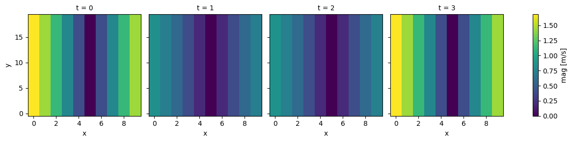
ds.mag.plot(col="t", x="x")

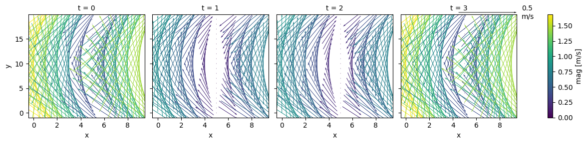
fg = ds.plot.quiver(x="x", y="y", u="u", v="v", col="t", hue="mag", scale=1)  # type: ignore[call-arg]

from pivpy import io, pivpy, graphics
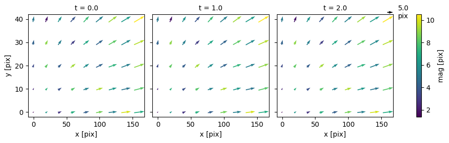
ds = io.create_sample_Dataset(n_frames=3,rows=5,cols=9,noise_sigma=0.2)
ds["mag"] = (ds["u"] ** 2 + ds["v"] ** 2) ** 0.5

# using default xarray.plot.quiver
fg = ds.plot.quiver(x="x", y="y", u="u", v="v", col="t", hue="mag", scale=100)  # type: ignore[call-arg]

# using overloaded pivpy graphics.quiver
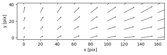
ds.piv.quiver(scalingFactor=100)

(<Figure size 640x480 with 1 Axes>, <Axes: xlabel='x [pix]', ylabel='y [pix]'>)